How Much Safety Stock Do You Really Need?
Safety stock is the inventory you carry above expected demand to protect against forecast error and late supply until the next replenishment arrives. If demand and lead time both move around, most planners use z × √(L × σe² + d² × σL²). For an item selling 900 cases a week, with 240 cases of weekly forecast error and a three-week lead time that varies by about two days, a 95% cycle service level works out to roughly 815 cases.
It’s a tidy number, and it can be badly wrong. A planning team can audit every safety stock setting in the ERP, confirm that each one was calculated correctly, and still finish the summer with two distribution centers short and a third holding six weeks of the same product. The arithmetic was fine. The inputs, and the assumptions underneath them, were not.
This guide covers the formulas, how to choose their inputs, how service levels turn into cash, and where the formula stops describing a food or beverage supply chain.
What does safety stock protect against?
Between placing an order and receiving it, two things can go wrong: customers buy more than expected, or the stock turns up late. Safety stock is there for both. It sits on top of cycle stock, which covers the demand you do expect before the next delivery. Stock you build on purpose, such as a pre-build ahead of a holiday peak, is neither. Counting it as safety stock makes the buffer look inflated for the rest of the year.
Mistakes cost money either way. Under-buffering shows up as short shipments, retailer fines, rush freight and slowly shrinking shelf space. Over-buffering shows up as cash sitting in cold storage and, for anything with a code date, as write-offs.
The four safety stock formulas
In practice, planners choose between four versions of the calculation. Each one models demand over the lead time as roughly bell-shaped and adds enough stock to cover z standard deviations above the expected level.
The worked example uses a foodservice case of frozen pizzas held at a regional distribution center (DC). It sells 900 cases a week on average. The standard deviation of weekly forecast error is 240 cases. Replenishment takes three weeks, with a standard deviation of 0.3 weeks. The target is a 95% cycle service level, so z = 1.645. The inputs are illustrative.
| Formula | Expression | Assumes | Example result |
|---|---|---|---|
| Demand uncertainty only | z × σe × √L | Lead time is fixed | 684 cases |
| Lead-time uncertainty only | z × d × σL | Demand is steady | 444 cases |
| Combined, independent | z × √(L × σe² + d² × σL²) | Both vary, for unrelated reasons | 815 cases |
| Combined, dependent | (z × σe × √L) + (z × d × σL) | Both vary, and move together | 1,128 cases |
For comparison, a “two weeks of cover” rule would hold 1,800 cases, more than twice the default. Rules based on weeks of cover give a steady item and a volatile item the same protection, so they overstock some products and understock others at the same time.
If the DC orders on a fixed weekly schedule rather than whenever stock falls to a trigger, the buffer also has to cover the week between orders. That raises the example to 906 cases. The reorder point is expected demand over the lead time plus safety stock: 2,700 + 815 = 3,515 cases.
Which formula should you use?
For most items, start with the combined, independent version. The demand-only version is enough when supply is dependable, for example a plant that ships to its own DC on the same days every week.
The dependent version belongs where one event drives both problems, and in food and beverage that is common. A heat wave lifts demand for drinks in the same weeks it stretches co-packer capacity and refrigerated trucking. The run-up to a holiday lifts demand while plants run flat out. Rules of thumb are useful as a cross-check, not as the policy.
Which standard deviation belongs in the formula?
Forecast error, not demand variability. The buffer is there for the misses, not for the swings the forecast already sees coming.
The difference is largest for seasonal items. A canned iced tea might sell 400 cases a week in January and 2,000 in July. The standard deviation of weekly demand across the year is about 565 cases. A reasonable forecast expects summer, so the error around it might be 150 cases. Put the first number into the formula and the DC carries close to four times the buffer it needs, all winter.
Three rules keep the input honest:
- Measure the error where the stock sits. Use error at SKU × location, not at product family or national level, where misses in one region cancel misses in another.
- Use the right lag. With a three-week lead time, score the forecast made three weeks before the period, not the version revised the day before.
- Deal with bias separately. A forecast that runs 8% light every week can show a small standard deviation and still empty the shelves. A bigger buffer is the wrong fix for a biased forecast.
If your system only keeps mean absolute deviation (MAD), multiply it by about 1.25 to estimate σ. The conversion holds as long as errors are roughly normal.
Where is the uncertainty coming from?
The two terms under the square root show which lever matters. In the example, forecast error contributes 172,800 to the variance and lead-time variability contributes 72,900, so forecast error accounts for 70% of the uncertainty.
That tells you where to spend effort. A 30% reduction in forecast error lowers safety stock from 815 cases to 653, a cut of 20%. Halving lead-time variability lowers it to 719, a cut of 12%.
For this item the forecast is the bigger lever. That pattern is typical in food manufacturing, where plants usually sit close to their DCs and internal lead times are short and fairly predictable. Items built on imported ingredients or long ocean lanes can flip it, which is why the split is worth running for the 100 SKU-locations that carry the most inventory value.
Choosing a service level
z comes from the service level, and each step up costs more than the last. At an illustrative $62 a case and a 25% annual carrying rate:
| Cycle service level | z | Safety stock | Inventory value | Annual carrying cost |
|---|---|---|---|---|
| 90% | 1.28 | 635 cases | $39,400 | $9,800 |
| 95% | 1.64 | 815 cases | $50,600 | $12,600 |
| 98% | 2.05 | 1,018 cases | $63,100 | $15,800 |
| 99% | 2.33 | 1,153 cases | $71,500 | $17,900 |
| 99.9% | 3.09 | 1,532 cases | $95,000 | $23,700 |
Going from 95% to 99% means 338 more cases. That is about $20,900 of inventory and $5,200 a year to carry, and it is one SKU in one building. Repeat it across 100 similar SKU-locations and the decision is worth roughly $2.1 million of working capital. Choosing between those two percentages is really choosing how much cash to park in a product line, and finance belongs in that conversation.
There is a textbook way to frame it. The cost-minimizing service level comes from the critical ratio, Cu ÷ (Cu + Co). Cu is what a missing unit costs you, usually the lost margin plus any penalty. Co is what a surplus unit costs you. When an unsold case simply carries into next week, Co is a few cents of carrying cost and the ratio is high: $14 of lost margin against $0.30 of carrying cost justifies about 98%. When an unsold case will be written off, Co becomes the full cost of the product, and the right answer can fall to around 50%.
Cycle service level and fill rate are not the same thing
Cycle service level is the chance of getting through a replenishment cycle without running out. Fill rate is the share of ordered cases shipped from stock. Many retail and foodservice agreements are written as fill rates, and mixing the two up is one of the most common sources of excess stock. For the example item, hitting a 99% fill rate takes about 844 cases. Setting the system to a 99% cycle service level instead holds 1,153, which is 37% more than the contract requires.
Where the formula stops working
Behind the formula sit four assumptions. Check them against a single DC’s history and you will usually find at least one that doesn’t hold.
Demand is assumed to be bell-shaped. For fast movers measured nationally, that is close enough. At a single DC, many items see weeks of nothing followed by a large foodservice or ingredient order. A symmetric curve can’t describe that pattern, and the result is stock that does nothing for weeks and then isn’t enough on the day it’s needed. For these items, build the buffer from the actual distribution of lead-time demand in your history.
Supply delays are assumed to be independent of demand. In practice the busiest weeks for demand are often the worst weeks for supply, because suppliers, co-packers and carriers are serving the same peak. Neither formula captures that well: one assumes no link, the other assumes a perfect one.
Every location is assumed to manage its risk alone. Safety stock at four regional DCs is calculated as if each had to cover its uncertainty without help. In reality, errors partly cancel across locations, products substitute for one another, and stock moves between sites. A single-item formula sees none of that, so the network as a whole carries more than it needs.
Past sales are assumed to equal demand. This is the assumption that does the most lasting damage. A sales history is a record of shipments. In a week when the DC ran out on Tuesday, the history shows Tuesday’s stock level as that week’s demand. When a constrained product is allocated across customers, each customer’s history shows them wanting less. The items that ran short most often end up looking calmer and smaller than they are, and they are the ones that most need protection (Nahmias, 1994). The next calculation lowers their buffer, they run short again, and the constraint becomes part of the forecast.
Food adds a fifth limit: shelf life. Every case starts aging when it is made, and many retailers only accept product with a minimum share of its life remaining. That gives each DC a sellable window:
Sellable window = shelf life − days before reaching the DC − customer’s minimum remaining shelf life
A chilled hummus with a 42-day shelf life that reaches the DC two days after production, for a retailer requiring 24 days remaining, has a 16-day window. The oldest case at the DC has waited roughly the days between production runs plus the safety stock in days of demand. A main flavor made weekly peaks at about nine days and fits. A slow flavor made every two weeks to save changeovers peaks at about 19 days, so part of every batch ages out however carefully the buffer is set. The constraint is production frequency, not safety stock.
Why do planners override the formula?
Planners hold information no formula has access to: a co-packer that has been late three times this quarter, a retailer planning to cut a flavor at the next shelf review, a sales team that has promised a new distributor launch volumes in writing. Their overrides are often right.
What goes wrong is the record keeping. A hand-typed buffer carries no explanation. Six months later nobody remembers why it was raised, whether the reason still applies, or whether it prevented a shortage or just added stock. The next recalculation may quietly overwrite it, and when the planner moves on, the knowledge goes with them. An override worth making is worth recording as an assumption with a reason and a review date, so it can be checked against what actually happened.
What AI changes about safety stock
That depends on which kind of AI is meant. Three quite different things are sold under the label.
Automation recalculates the same buffer more often. Many tools labelled AI simply run the existing calculation on a tighter schedule and route the exceptions to a planner. Planners get time back. The buffers themselves are no better: if lumpy demand made a buffer wrong yesterday, a nightly recalculation just makes it wrong on schedule.
Better forecasting improves the inputs. A model trained on a company’s own history, network and outside signals can estimate demand and its uncertainty for each item at each location far more precisely than a statistical method fitted to one series at a time. Because safety stock moves almost in proportion to forecast error for most food items, this is where the largest gains usually sit today.
Decision models choose the stock position directly. Research has shown that learning the stocking decision straight from data, rather than estimating a demand distribution and plugging it into a formula, can produce better inventory decisions (Bertsimas and Kallus, 2020). These approaches are promising, and they still depend on the same foundation: demand data that reflects what customers wanted rather than what the business was able to ship.
Whichever approach you use, choosing the service level remains a judgment about the business. Good tools show what each choice costs. People should still make it.
Signs your safety stock is set by the wrong math
- Service misses in both directions. Some items run well below their target while others beat it comfortably, which means the inputs, not the targets, are off.
- The source of σ is a mystery. If nobody can say whether the standard deviation comes from demand history or forecast error, or from which period, the buffers can’t be trusted.
- The same product line is both short and overstocked. One DC writes off what another can’t get.
- Hand-edited buffers outnumber calculated ones. At that point the formula is a starting suggestion, not the policy.
- Last season’s shortages are in this season’s inputs. When an item ran out, its recorded demand fell, and the recalculated buffer got smaller.
- Fresh items run past their sellable window. Production frequency, not the buffer, is the binding constraint.
If two or more sound familiar, the next step isn’t a new formula. Pull every buffer a planner has changed by hand in the last six months and compare it with the calculated value. Where the planner was right, the formula is missing information. Where the formula was right, the override is costing money.
How Daisy helps
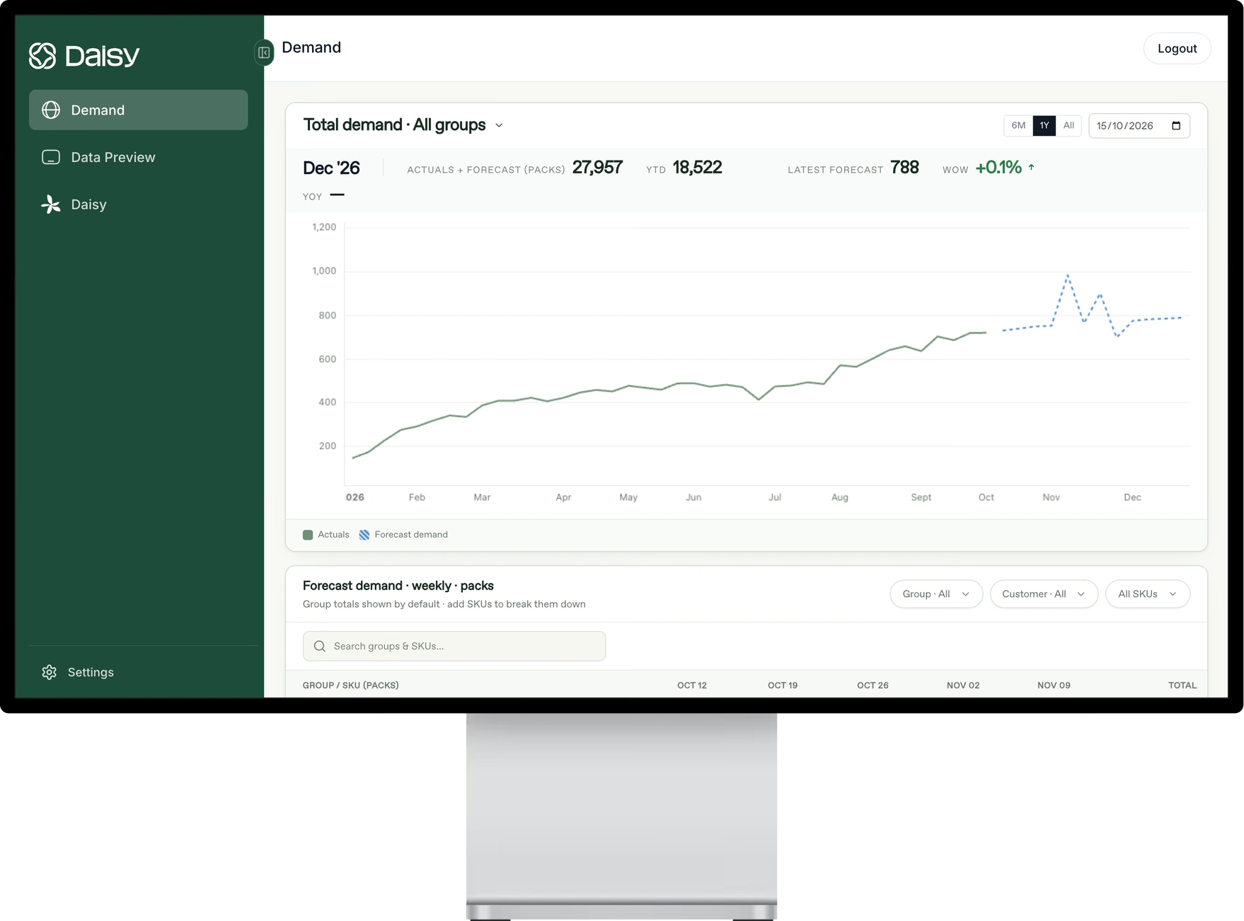
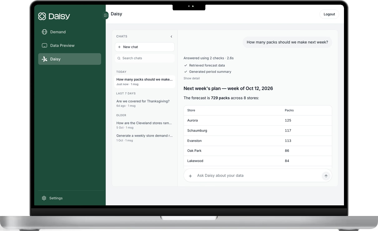
Every version of the formula depends on σ, and σ is forecast error at the location where the stock sits. Daisy builds a forecasting model for each manufacturer, trained on that company’s own plants, DCs, customers and products, and on thousands of external signals such as weather, holidays and category trends. It forecasts at SKU × location × account, the level where safety stock is actually set, and it doesn’t require your data to be cleaned first.
Each forecast comes with the drivers behind it, so a planner can see why an item’s uncertainty is high and act on it, instead of padding a number in a spreadsheet. Kerry Dairy Ireland replaced a spreadsheet-based forecasting process with Daisy, cut its annual forecasting margin of error by up to 60%, and now produces its forecast ten times faster. Read the case study.
Frequently asked questions
What is the safety stock formula?
Most planners use z × √(L × σe² + d² × σL²). It sizes the buffer to cover forecast error and supply variability during the lead time, at the confidence level set by z.
How is safety stock different from the reorder point?
Safety stock is protection: stock held on top of what you expect to sell. The reorder point is a trigger: when stock on hand plus stock on order falls to it, you reorder. It equals expected lead-time demand plus safety stock.
Should the formula use demand variability or forecast error?
Forecast error for that item at that location, using the forecast made one lead time ahead. Raw demand swings include patterns a good forecast already expects, so they exaggerate the risk.
What service level should I use?
Let the economics decide: what a shortage costs you against what an extra unit costs to hold or write off. Read the customer contract first, too. A fill-rate commitment usually needs less stock than the same percentage set as a cycle service level.
How do you set safety stock for perishable products?
Calculate the buffer as usual, then check it against the sellable window. If the days between production runs plus the safety stock in days of demand exceeds the window, change production frequency or reduce forecast error before raising the buffer.
How often should safety stock be updated?
Monthly is a sensible minimum, and seasonal items need their buffers reset as the season moves. Any big change, such as a new DC, a new supplier or a lost customer, is a reason to recalculate straight away.
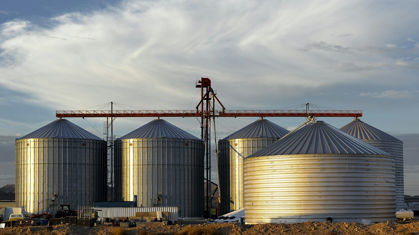
Photo: Jim Witkowski on Unsplash.
See Daisy in action.
Ready to implement in 2 weeks
Want to try Daisy?
We’ll be in touch shortly to set up a time.