How to Calculate Forecast Accuracy, and Which Number to Trust
Forecast accuracy is usually reported as 1 − WAPE: one minus the total absolute error divided by total actual demand. But the same forecast for the same month can score anywhere from 53% to 97% depending on the formula, the level of detail and the forecast version you choose. Those choices, made before any arithmetic, decide whether the number tells you anything.

A monthly business review shows forecast accuracy at 96.7%, the best in two years. In the same month, one distribution center ran out of the company’s best-selling SKU for nine days and another wrote off a pallet of seasonal product. Both facts are true. The accuracy figure was measured across the whole company, where Chicago’s over-forecast cancelled Dallas’s under-forecast. The trucks, unfortunately, went to Chicago and Dallas.
This guide works through the common metrics on one small dataset, with the Excel formula for each, then covers how to test a forecast fairly and why a healthy accuracy number can hide a business that is constraining itself.
Three choices to make before you calculate
- The level. Accuracy for the whole company, a product family, a SKU, or a SKU at one DC are four different measurements. Errors cancel as lines are added together, so higher levels always look better. The level that counts is the one where inventory and production decisions are made, usually SKU × location.
- The lag. Score the forecast that existed when the decision was made. If a product takes three weeks to plan, make and ship, score the forecast made three weeks before the period. A version revised the day before will look excellent and drove nothing.
- The sign. This guide uses error = forecast − actual, so a positive number means you over-forecast. Pick one convention and print it on every report.
The worked example
A beverage and snack manufacturer ships four SKUs from two DCs. Here is September, using the forecast made one month ahead. The numbers are illustrative.
| SKU | DC | Forecast | Actual | Error |
|---|---|---|---|---|
| Sparkling water 12-pack | Chicago | 4,200 | 3,850 | +350 |
| Sparkling water 12-pack | Dallas | 2,900 | 3,310 | −410 |
| Cold brew 4-pack | Chicago | 1,800 | 1,640 | +160 |
| Cold brew 4-pack | Dallas | 1,250 | 1,020 | +230 |
| Protein bar 12-count | Chicago | 600 | 710 | −110 |
| Protein bar 12-count | Dallas | 380 | 300 | +80 |
| Holiday spice syrup | Chicago | 40 | 12 | +28 |
| Holiday spice syrup | Dallas | 25 | 0 | +25 |
| Total | 11,195 | 10,842 | +353 |
The Excel formulas below assume forecasts are in C2:C9 and actuals in D2:D9.
MAPE: the familiar one
MAPE = average of ( |forecast − actual| ÷ actual )
Leaving out the Dallas syrup line, where the actual is zero and the percentage can’t be calculated, MAPE is 47.0%, which suggests the forecast is only 53% accurate. Drop both syrup lines and it falls to 16.0%. A seasonal SKU that sold 12 cases in Chicago has moved the headline by 31 points.
That is the core weakness of MAPE. Every line counts equally, so small items with large percentage misses dominate, and a zero actual breaks the calculation entirely. It is also lopsided. An under-forecast can never produce an error above 100%, but an over-forecast can, so a team judged on MAPE learns to forecast light. MAPE works for comparing similar, high-volume items. As a portfolio headline it misleads.
In Excel: =AVERAGE(IF(D2:D9<>0, ABS(C2:C9-D2:D9)/D2:D9)), confirmed with Ctrl+Shift+Enter in versions before Microsoft 365.
WAPE: the one to report
WAPE = Σ |forecast − actual| ÷ Σ actual = 1,393 ÷ 10,842 = 12.8%
Forecast accuracy is then 1 − WAPE, or 87.2%. WAPE weights each line by its volume, so the lines that move the most product count the most. The two syrup lines contribute 53 cases of error out of 1,393, roughly their real importance. WAPE handles zeros, holds up at SKU × location level, and is the best single headline for most food and beverage portfolios. You will also see it called weighted MAPE or the MAD/mean ratio.
In Excel: =SUMPRODUCT(ABS(C2:C9-D2:D9))/SUM(D2:D9)
Where low-volume items carry high value, weight by value instead. With illustrative prices of $38, $52, $44 and $95 a case, value-weighted WAPE is 13.7%. With prices in E2:E9: =SUMPRODUCT(ABS(C2:C9-D2:D9)*E2:E9)/SUMPRODUCT(D2:D9*E2:E9)
Bias: which way you missed
Bias = ( Σ forecast − Σ actual ) ÷ Σ actual = 353 ÷ 10,842 = +3.3%
Error tells you how far off you were. Bias tells you which way, and the direction is what decides whether a warehouse fills up or runs dry. A forecast can post a respectable WAPE and still run 3% heavy every month, building excess inventory by design. Report bias next to accuracy, always, and at the same level: the total can look neutral while one DC runs heavy and another light.
In Excel: =(SUM(C2:C9)-SUM(D2:D9))/SUM(D2:D9)
One month proves little. The tracking signal, cumulative error divided by mean absolute deviation, tests whether misses keep leaning the same way. A common rule is to investigate when it moves outside ±4. An item whose monthly errors run +120, +80, +150, −30, +110 and +90 crosses that line in month five. No single month looked unusual. Together they describe a forecast that runs high.
MAE and RMSE: error in units
MAE, the average absolute error, is 174 cases. RMSE, the square root of the average squared error, is 221 cases. Both are in units, which makes them useful within one item and misleading across items of different sizes. RMSE punishes big misses harder, so when it sits well above MAE, a few large errors are doing most of the damage. RMSE is also the closest relative of the standard deviation that goes into a safety stock calculation.
In Excel: =SUMPRODUCT(ABS(C2:C9-D2:D9))/COUNT(D2:D9) for MAE, and =SQRT(SUMXMY2(C2:C9,D2:D9)/COUNT(D2:D9)) for RMSE.
Is the forecast beating a naive guess?
A naive forecast repeats the last period’s actual, or for seasonal products, the same period last year. It costs nothing, so every forecasting process should beat it. Using August’s actuals as the naive forecast for September gives a WAPE of 16.3%, against 12.8% for the company’s forecast.
The forecast adds 3.4 points of accuracy. That is worth having, and it is a lot less impressive than the 87% headline. The same comparison should be run on every step of the process: the statistical baseline, the planner’s adjustments, the consensus number agreed in the demand review. This is forecast value added. Any step that doesn’t beat the one before it is costing time and accuracy, and should be changed or removed.
Same forecast, four different numbers
Now add the lines together in different ways and recalculate 1 − WAPE:
| Measured at | Accuracy |
|---|---|
| SKU × DC (the eight lines) | 87.2% |
| SKU (both DCs combined) | 95.1% |
| DC (all SKUs combined) | 95.4% |
| Company total | 96.7% |
Nothing about the forecast changed. Chicago’s over-forecast on sparkling water offset Dallas’s under-forecast, so the SKU total was only 60 cases off. Report the aggregate if leadership wants it, but never on its own. The number that predicts inventory and service is the one measured where the stock sits.
How to test a forecast fairly
Most in-house comparisons of forecasting methods, and many vendor pilots, are set up, often unintentionally, to make the winner look better than it is. A few rules prevent that.
Use a rolling back-test. Train on everything up to a cut-off date, forecast the period after it, then push the cut-off forward a period and do it again. Every score then comes from data the model had no chance to learn from. A single holdout is easy to overfit: tune a model against the same months you score it on and the result describes those months, not the future. Pilots that report a spectacular number and then disappoint in production usually got there this way.
Score at the level and lag you plan at. A model evaluated nationally by month and deployed by DC and week hasn’t really been evaluated.
Include the hard cases. Removing promotions, launches and “unforecastable” weeks after the fact removes the most expensive part of the job. Report them separately if you like, but count them.
Always compare with a simple benchmark. It is surprisingly hard to beat. In the M4 forecasting competition, which covered 100,000 time series with no explanatory data attached, the most accurate entries were mostly combinations of statistical methods, and pure machine learning entries performed poorly (Makridakis, Spiliotis and Assimakopoulos, 2020). In the later M5 competition, built on Walmart sales with prices, promotions and calendar data included, machine learning methods took the top places and the winner beat the best statistical benchmark by more than 20% (Makridakis, Spiliotis and Assimakopoulos, 2022). The lesson is consistent: sophisticated methods win when there is real information beyond the shape of the history to learn from, and lose to a well-chosen simple method when there isn’t.
Why a healthy accuracy number can hide a constrained business
Accuracy is measured against actuals, and actuals are shipments. When an item was out of stock, shipments understate what customers wanted. When product was allocated during a shortage, each customer’s history shows them wanting less. A forecast that predicts those constrained shipments scores well, because the forecast and the shortage came from the same plan.
If last year’s sales were capped by what you could supply, a forecast that simply repeats the cap will look accurate. Buy to it, hit the cap again, and the next forecast learns an even tighter record. The accuracy report ends up agreeing with the plan rather than checking it. That is why accuracy should always be read alongside service, lost sales and stockout days, and why a forecasting system needs to know which parts of the history were customer decisions and which were yours.
What is a good forecast accuracy?
There is no industry benchmark worth quoting. Accuracy depends on the level, the lag, how volatile the category is, how much volume runs on promotion and how many new products are in the mix. Three comparisons tell you more:
- Against naive. If you aren’t clearly beating a seasonal naive forecast, nothing else matters yet.
- Against your own trend. Is accuracy at your planning level improving quarter by quarter, at the same lag?
- Against the cost of error. Multiply absolute error by unit cost. In the example, 1,393 cases of error is about $62,600 of product in the wrong place or not made at all, in one month, across just eight lines.
Signs your accuracy reporting is misleading you
- The headline is measured at company or family level. Offsetting errors make it look better than any DC experiences.
- It is scored at lag zero. The last revision before the period wins, and nobody acted on it.
- MAPE is the headline across a long tail. A handful of small items is driving the number.
- Promotions and launches are excluded. The hardest, most expensive forecasts are missing from the score.
- Accuracy rose but service and inventory didn’t. The metric is measuring something the business doesn’t use.
- Nobody tracks value added by step. Overrides and consensus changes might be helping or hurting, and no one knows which.
How Daisy helps
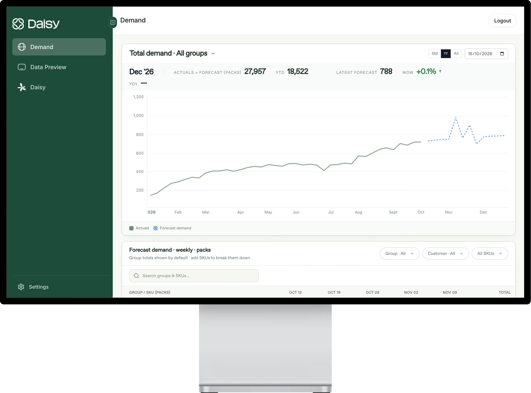
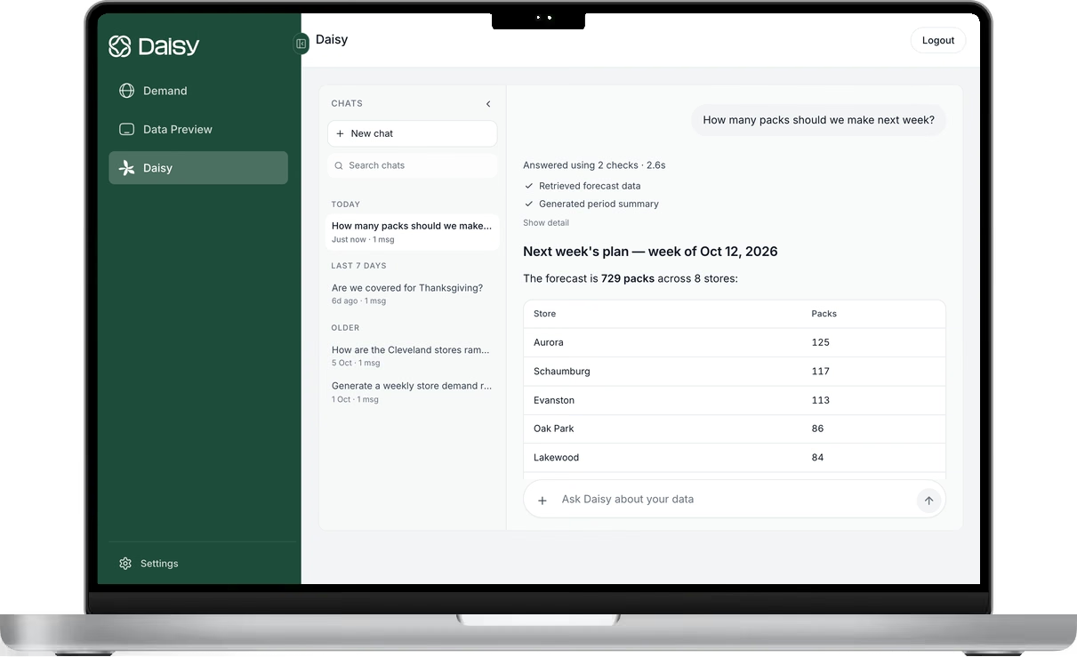
Daisy is measured the way this guide recommends: at the level forecasts are used, SKU × location × account, against your current forecast and on your own data. During a pilot, both forecasts are scored on the same actuals, so the comparison is fair before you commit.
Daisy builds a model for each manufacturer, trained on that company’s own network and on thousands of external signals, and explains the drivers behind every forecast, so when error moves, planners can see why. Kerry Dairy Ireland reduced its annual forecasting margin of error by up to 60% with Daisy and now produces its forecast ten times faster. Read the case study.
Frequently asked questions
How do you calculate forecast accuracy?
Use 1 − WAPE, where WAPE is the sum of absolute errors divided by the sum of actuals. Calculate it at the level you plan and purchase at, using the forecast made one lead time before the period.
What is the difference between MAPE and WAPE?
MAPE averages the percentage error of each line, so small items with large percentage misses can dominate and zeros break it. WAPE divides total absolute error by total actual demand, so each line counts in proportion to its volume.
What is forecast bias?
Whether a forecast runs consistently high or low: (sum of forecasts − sum of actuals) ÷ sum of actuals. A positive result means over-forecasting. Track it at the same level as accuracy, because offsetting errors can hide it in totals.
What is forecast value added?
A comparison of each step in the forecasting process against the one before it and against a naive benchmark. Steps that don't improve accuracy are costing time and should be changed or removed.
Why is our forecast accuracy high but we still have stockouts?
Usually because accuracy is measured at too high a level or too short a lag, or against shipments that were themselves constrained by stockouts. Recalculate at SKU × location, at the lead-time lag, and read it alongside service.
Does machine learning always forecast more accurately?
No. It tends to win when demand depends on drivers it can learn from, such as price, promotions and distribution, and to lose to well-chosen simple methods when the history is short or the drivers aren't recorded.
Photo: Alex Wigan on Unsplash.
See Daisy in action.
Ready to implement in 2 weeks
Want to try Daisy?
We’ll be in touch shortly to set up a time.