Inventory Optimization: How Food Manufacturers Free Up Cash Without Cutting Service
Inventory optimization means deciding how much of each product to keep at each site, and when to top it up, so that customers get the service they were promised for the least cash and cost. In a food or beverage business it covers production run sizes, reorder points, safety stock, where buffers sit in the network, and which products deserve which service level.
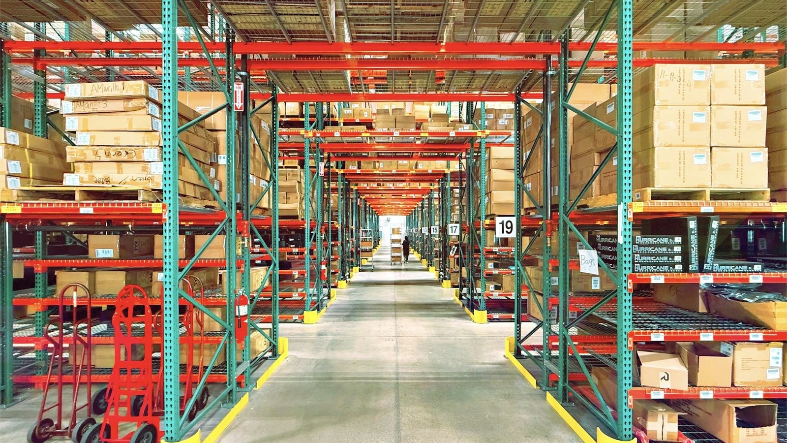
Several neighboring terms cause confusion. Inventory management is the physical side: receiving, storing, counting and shipping. Replenishment is the act of ordering. Multi-echelon inventory optimization (MEIO) is a specialist technique for networks with several tiers of stock. Inventory optimization is the set of decisions that tells all of those activities what to aim for.
Why does inventory optimization matter?
For most manufacturers, inventory is the biggest block of cash they can actually influence, and mistakes are expensive whichever way they go.
Take a food manufacturer with $400 million in revenue, $300 million in cost of goods sold (COGS) and $55 million of inventory at cost. That is 67 days of inventory, or about 5.5 turns a year. Holding it costs more than the cost of capital. It includes refrigerated and frozen storage, handling, insurance, and the write-offs that come with code dates. Many food manufacturers plan on 20% to 30% of inventory value a year. At 25%, that inventory costs about $13.75 million a year to carry.
Cut it by 15% without losing service and the business releases $8.25 million of cash once and saves about $2 million every year after. Get it wrong the other way and the bill arrives as retailer fines, expedited freight, overtime and lost shelf space.
Most of the excess on a food company’s balance sheet traces back to one of two things moving: the mix of what customers bought, or how long supply took to arrive. The standard methods assume both stay put.
The classical toolkit
The methods most manufacturers run today were developed over the last century. They run in seconds, and any planner can walk you through the result. That transparency is why they are still everywhere.
Run size: EOQ and EPQ
The economic order quantity (EOQ) trades off the fixed cost of each order against the cost of carrying the stock it brings in. Manufacturers sizing their own production runs use its close relative, the economic production quantity (EPQ), which accounts for stock building up gradually while the line runs:
EPQ = √( 2 × annual demand × changeover cost ÷ ( holding cost × ( 1 − demand rate ÷ production rate ) ) )
For a chilled hummus flavor selling 52,000 cases a year, with a $900 changeover (flush, lost line time, product loss and labor) and a $3 annual holding cost per case, EPQ is about 6,000 cases, roughly six weeks of demand. For a shelf-stable product that would be a reasonable answer. For hummus with a 42-day shelf life and retailers that want most of it remaining on delivery, it is impossible. Runs have to be closer to one week.
| Policy | Changeovers per year | Annual cost |
|---|---|---|
| Textbook EPQ (about six weeks per run) | 9 | $15,600 |
| Weekly runs, $900 changeover | 52 | $48,100 |
| Weekly runs, changeover cut to $450 | 52 | $24,700 |
Shelf life costs this one SKU about $32,500 a year against the textbook answer, and halving the changeover cost wins back $23,400 of it. In fresh categories, the real optimization lever is the cost of each changeover: sequencing flavors from light to dark, running allergen-free products first, and grouping SKUs that share a base.
Reorder points and safety stock
The reorder point tells you when to replenish: expected demand over the lead time plus safety stock. Safety stock covers forecast error and late supply during that lead time. The standard formula, z × √(L × σe² + d² × σL²), and the assumptions behind it are covered in detail in the companion guide, How Much Safety Stock Do You Really Need?
Service levels by segment
The z in that formula comes from a service target, and one target for the whole portfolio guarantees that some items carry too much stock and others too little. Most companies segment by value (ABC) and by how forecastable each item is (XYZ), then set a target for each group:
| X: forecastable | Y: variable | Z: erratic | |
|---|---|---|---|
| A: high value | 98–99% | 97–98% | 95–97% |
| B: mid value | 96–97% | 95% | 90–93% |
| C: low value | 93–95% | 90% | 80–85%, or make to order |
These are starting points. Fresh products need one more adjustment: when surplus will be written off rather than sold next week, cap the target at what the item’s margin can justify.
Multi-echelon optimization and pooling
Calculating each site’s buffer separately misses the fact that forecast errors at different sites partly cancel out. A SKU held at four regional DCs, each with weekly error of 150 cases and a two-week lead time, needs about 1,400 cases of safety stock in total at a 95% target. One central DC needs about 700 if regional demand varies independently, or about 1,100 if regions tend to move together. The general result, that total buffer grows with the square root of the number of stocking points, has been known since the 1970s (Maister, 1976). MEIO methods build on it to place buffers across tiers. Often the answer is to keep more stock at a central or plant DC, where a single case can back up several regional sites, and less at the edges.
Food has costs on the other side of that trade: longer delivery distances, shelf life used up in transit, and cold chain freight. The usual compromise is to hold fast movers close to customers and pool slow movers centrally, where the saving is largest.
Mathematical optimization
Some manufacturers go further and describe the whole network as a linear or mixed-integer program. Instead of sizing each buffer separately, the program decides production, storage and shipments together to minimize total cost within the network’s limits. Some limits can never be broken, like a line’s maximum output. Others can be broken at a price, like a preferred minimum run. A solver finds the best plan for the model it is handed, which makes the quality of that model, and how up to date it is, the whole question.
How to tell whether inventory is working
Any single inventory metric can be improved by damaging another, so judge them in pairs:
- Days of inventory or turns, read alongside fill rate or on-time, in-full (OTIF) delivery
- Write-offs and aged stock, read alongside stockouts at SKU × location
- Expedite and freight spend, a sign that stock is in the wrong building even when the total looks fine
- Forecast accuracy where the stock actually sits, read alongside forecast bias
Report at SKU × location as well as in total. Company-wide figures can hide excess and shortage in the same product family, sometimes in the same week.
Where do the classical methods break?
None of these methods is wrong. They are approximations, and food and beverage networks stretch them in predictable places. The giveaway is how planners talk about their buffers: there is the number the system calculated, the number they actually hold, and a list of reasons for the difference that the system knows nothing about. Most of that list falls into four groups.
Demand isn’t well behaved at the level where decisions are made. A bell curve describes a fast mover nationally. At a single DC, many items are intermittent or skewed, so formulas set buffers too thin for some products and too heavy for others.
Sales history isn’t demand history. When an item ran out, the history shows what was on the shelf, not what customers wanted. When product was allocated during a shortage, each customer’s history shows them wanting less. Anything trained on that record inherits the shortages as if customers had chosen them, buys less next time, and creates the next shortage. Each cycle, the business plans for slightly less than it could have sold (Nahmias, 1994).
Shocks don’t arrive one at a time. Standard formulas treat demand and supply variability as unrelated. A heat wave, a port closure or a tariff deadline hits demand and supply in the same weeks, across many products at once. Buffers sized as if those were separate events are thinnest when the pressure is highest.
The forecast is graded on the wrong test. In most planning stacks, one step produces the most accurate forecast it can and a separate step treats that forecast as fixed. But misses are not equally expensive. Ten cases too many of a low-margin, long-life sauce costs a little storage. Ten cases too few of a high-margin seasonal item in its peak week costs the sale, the retailer’s goodwill and possibly the next promotion slot. Accuracy metrics score those two misses the same. The business doesn’t.
Planners patch these gaps one item at a time, and every patch makes sense. The cumulative effect is that the policy the business actually runs is no longer in any system. It is spread across workbooks and memories, it can’t be tested, and it walks out the door with the people who built it.
How is AI changing inventory optimization?
In two very different ways, and the difference matters more than the label.
Doing the same job faster
A lot of what is marketed as AI for inventory speeds up the existing routine: nightly recalculations, exception alerts, draft purchase orders, a chat window for questions. The time saving is real. It is also limited by how many planners you employ, and it leaves the policy itself untouched. Refreshing a safety stock calculation nightly doesn’t stop it assuming demand is bell-shaped and that suppliers run late for reasons unrelated to demand.
Making a better decision
The larger opportunity is in the decisions themselves. Automation touches the hours planners spend. Better decisions touch every dollar of stock they manage. Research points in three directions. Training a forecasting model on the cost of the decisions it drives, rather than on accuracy alone, can produce better decisions (Elmachtoub and Grigas, 2022). Learning stocking decisions directly from data and outside signals can outperform the classic estimate-then-optimize approach (Bertsimas and Kallus, 2020). And learned policies have matched the best known heuristics on hard problems such as lost sales and multi-echelon networks (Gijsbrechts and colleagues, 2022).
In practice, the gains show up in a few specific ways: service targets set by the economics of each item rather than by blanket percentages; inventory and production decisions considered together; and planner knowledge entering the plan as an input that can be checked later, instead of as a manual buffer on one line.
What AI doesn’t change
Some things stay fixed whatever the software. Suppliers still need weeks to deliver, lines still need cleaning between allergens, product still carries a code date and warehouses still fill up. A good model represents those limits accurately rather than wishing them away. And for some companies, advanced planning isn’t the next step at all. A manufacturer with a short, steady catalog, one DC and dependable suppliers will capture most of the benefit with well-kept formulas and a regular review. The argument for doing more gets stronger as products, sites and volatility multiply, and as more of the real policy ends up in workarounds.
The biggest lever is the forecast
For most food items, safety stock moves almost in proportion to forecast error. Take a portfolio of 100 SKU-locations like the frozen pizza example in the safety stock guide, about $290 million a year of product at cost. At a 99% fill rate it needs about $5.2 million of safety stock. Cut forecast error by 30% and that falls to $4.0 million. Cut it in half and it falls to $3.3 million. Service doesn’t move and no policy changes. The business holds less because it is less uncertain.
The forecast shapes the other layers too. Cycle stock depends on how confidently you can commit to a run. Anticipation stock depends on how clearly you can see a peak coming. And a forecast with a persistent 5% upward bias builds 5% excess, quietly, month after month.
Signs your inventory policy has hit its ceiling
- Planners override calculated buffers as a matter of routine. The system’s numbers have become suggestions.
- A better forecast didn’t change the inventory. Accuracy went up and the stock position looks the same, because nothing downstream used the improvement.
- Excess and shortage sit side by side. The same product family is aged in one DC and short in another.
- Shortages make next year’s plan smaller. The weeks you ran out are teaching the forecast that nobody wanted the product.
- Your network settings are older than your network. New plants, DCs, co-packers or channels have arrived since anyone last updated the configuration.
- Every what-if is a project. Trying a different service target means a week in a spreadsheet, so it rarely happens.
If several of these apply, the constraint is the method, not the team.
How Daisy helps
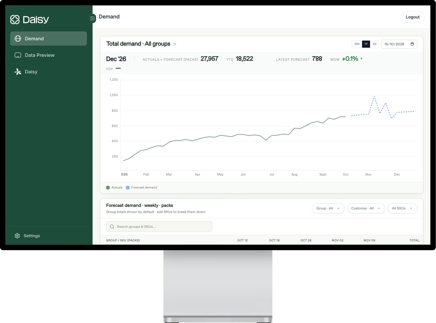
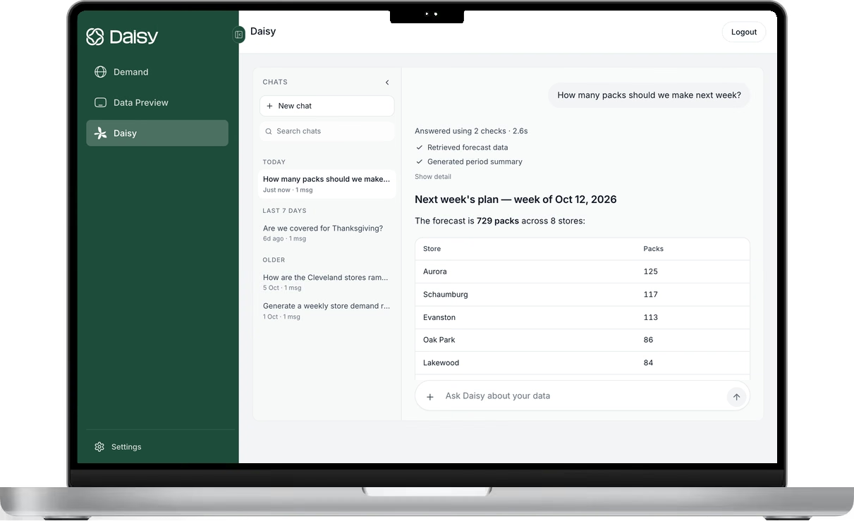
Daisy is built for the decision that inventory depends on most: the forecast at the level stock is held. It trains a model for each manufacturer on that company’s own network of plants, DCs, customers and products, and on thousands of external signals, and it forecasts at SKU × location × account. It works with your data as it is, without a cleaning project first.
Each forecast comes with the drivers behind it, so planners can see why a buffer is large and decide whether it should be. Kerry Dairy Ireland replaced spreadsheet-based forecasting with Daisy, reduced its annual forecasting margin of error by up to 60%, and now forecasts ten times faster. Read the case study.
Frequently asked questions
What is inventory optimization?
Setting stock levels item by item and site by site, along with run sizes and replenishment triggers, so customers get the service they were promised for the least cash and cost.
How is inventory optimization different from inventory management?
Management is doing: receiving, storing, counting and shipping. Optimization is deciding: how much of each item to keep at each site and when to reorder, so the doing is aimed at the right targets.
What is a good inventory turnover for a food manufacturer?
It depends on the category. A fresh business holding about a week of finished goods turns it roughly 50 times a year, while a business that ages product for a year may turn it once. Compare yourself with companies that share your shelf life and production model, and watch your own trend.
How does shelf life affect inventory optimization?
It caps run sizes and buffers, and it raises the cost of surplus from a few cents of carrying cost to the full cost of the product. That shifts the focus to shorter runs, cheaper changeovers and more accurate forecasts.
Does every manufacturer need AI for inventory?
No. With a small, steady catalog, one warehouse and reliable suppliers, well-kept formulas and a regular review capture most of the value. More advanced planning pays off as products, sites and volatility grow.
Photo: Russ Murray on Unsplash.
See Daisy in action.
Ready to implement in 2 weeks
Want to try Daisy?
We’ll be in touch shortly to set up a time.